
Contextual Embeddings
Understand why the same token ID can end up with different vectors: how the transformer turns a context-free lookup into a context-aware representation.
Contextual Embeddings: Clay Shaped by Its Neighbours
Every sentence hands the word bank the same lump of clay from the shelf. The surrounding words then shape it — loan pushes it one way, river the other. The shaping rules are the transformer weights learned in training.
IntroductionWhat is a contextual embedding?
"'The bank approved my loan' and 'We sat on the bank of the river' both contain the word bank. How can the AI tell them apart if the word is converted to the same number?"
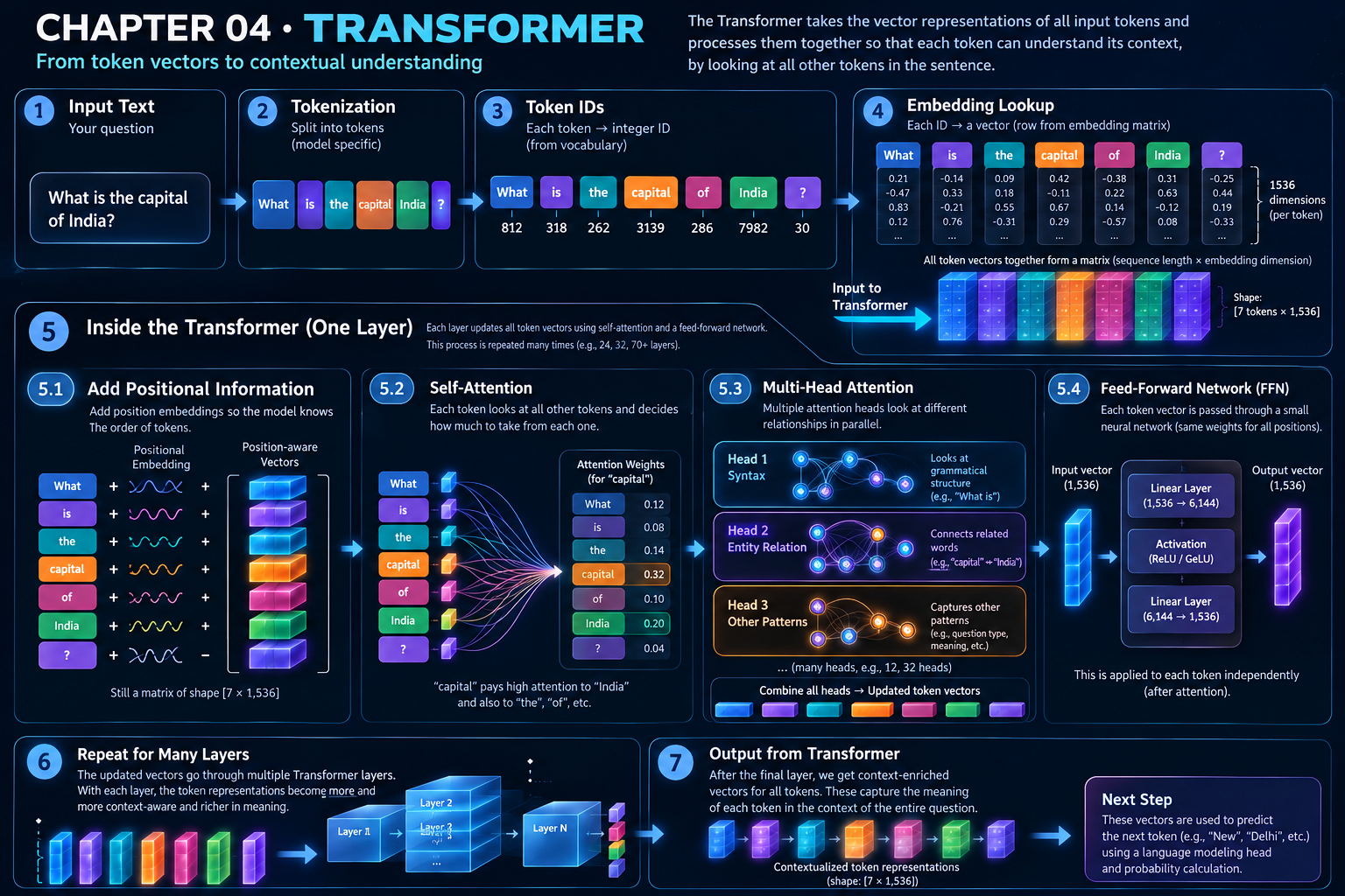
It can't — at the start. The token ID for bank is the same, and so is its embedding-matrix row. The difference appears after the transformer layers have let bank look at its neighbours.
bank the same starting vector. Each transformer layer then adjusts that vector using the other tokens in the sentence. By the end, the "financial" bank and the "river" bank are different vectors. Those updated vectors are contextual embeddings.
A contextual embedding (also called a contextual representation or hidden state) is a token's vector after the transformer has mixed in information from the surrounding tokens. A static token embedding is the context-free row read straight from the embedding matrix.
💡 Same ID in, different vector out. The token ID for bank can be identical in both sentences, but the transformer builds a different contextual representation for it from the surrounding words.
WhyWhy isn't the embedding lookup enough?
The lookup in Token Embeddings depends on one thing only: the token ID. Same ID, same row — always.
- Words are ambiguous: bank, bat, light, play.
- Meaning also changes through grammar and reference: "it" refers to different things in different sentences.
- Language models must predict the next token or answer questions about this sentence, not about the word in general.
Sentence A
"The bank approved my loan."
Neighbours such as approved and loan point to a financial institution.
Sentence B
"We sat on the bank of the river."
Neighbours such as sat and river point to land beside water.
IntuitionClay that gets shaped by its neighbours
Think of the embedding-matrix row as a lump of clay taken from the shelf. Every sentence that contains bank starts with an identical lump.
- In "The bank approved my loan", the neighbours
approvedandloanpress the clay toward a financial shape. - In "We sat on the bank of the river",
satandriverpress it toward a riverside shape. - The shaping rules — how strongly to listen to which neighbour — are the transformer's learned weights. They were fixed during training.
The full side-by-side walkthrough of this example lives on Static vs Contextual Embeddings. This page focuses on where it sits in the pipeline and shows a small calculation you can check by hand.
💡 Critical mental model: the lookup does not know the sentence. The transformer does the contextualising, using weights learned in training.
TheoryLayer by layer: from static to contextual
Write $\mathbf{h}_i^{(0)}$ for the vector a token has when it enters the first transformer layer, and $\mathbf{h}_i^{(\ell)}$ for its vector after layer $\ell$.
| Where | Notation | Depends on |
|---|---|---|
| After tokenization | token ID $t_i$ | Only the token's own identity |
| After embedding lookup | $\mathbf{h}_i^{(0)} = \mathbf{E}[t_i]$ (plus position information in most models) | The token ID (and its position) |
| After transformer layer $\ell$ | $\mathbf{h}_i^{(\ell)}$ | All tokens the layer can attend to |
| Final layer | $\mathbf{h}_i^{(L)}$ | The whole visible context, shaped by every layer |
Where the knowledge lives
- The learned parameters — the embedding matrix and the transformer weights — were established during training.
- At inference, the same fixed weights process every sentence. What changes from sentence to sentence is the input, and therefore the contextual vectors.
- So the model does not "gain" knowledge at the embedding stage; it applies what it already has to your tokens.
How It WorksTracing "bank" through two sentences
bank token with the same token ID (the ID is whatever your tokenizer assigns).bank tokens read the same row of the embedding matrix, so their starting vectors are identical.bank scores every other token, turns the scores into weights, and takes a weighted mixture of their information.bank vectors drift apart.
graph TD
    A["bank (ID is the same in both sentences)"] --> B["E[id] (same row)"]
    B --> C1["Sentence A: neighbours = approved, loan"]
    B --> C2["Sentence B: neighbours = sat, river"]
    C1 --> D1["Transformer layers"]
    C2 --> D2["Transformer layers"]
    D1 --> E1["bank: financial-leaning vector"]
    D2 --> E2["bank: riverside-leaning vector"]

    style A fill:#3b82f6,stroke:#1d4ed8,color:#fff
    style B fill:#10b981,stroke:#047857,color:#fff
    style E1 fill:#8b5cf6,stroke:#6d28d9,color:#fff
    style E2 fill:#f59e0b,stroke:#b45309,color:#fff
CalculateA two-dimensional toy you can check by hand
Imagine dimension 0 means "finance-ish" and dimension 1 means "nature-ish". These numbers are invented for teaching; real embeddings are not interpretable axis by axis.
bank = [0.5, 0.5] (ambiguous: equally finance and nature)loan = [0.9, 0.1]river = [0.1, 0.9]
0.707 and cos(bank, nature axis) = 0.707. The static vector cannot choose.[0.5, 0.5].New bank = 0.5·[0.5, 0.5] + 0.5·[0.9, 0.1] =
[0.7, 0.3]New bank = 0.5·[0.5, 0.5] + 0.5·[0.1, 0.9] =
[0.3, 0.7]Sentence A: cos with finance =
0.919, with nature = 0.394Sentence B: cos with finance =
0.394, with nature = 0.919cos(A's bank, B's bank) =
0.724 — same start, now different.
MathematicsAttention as a weighted mixture
In one simplified attention step, token $i$ builds a new vector from all tokens $j$:
- $\alpha_{ij}$ is how much token $i$ listens to token $j$; the weights over $j$ sum to 1.
- $\mathbf{q}, \mathbf{k}, \mathbf{v}$ are produced from the token vectors by learned weight matrices (see the Q/K/V roadmap topic).
- Because $\alpha_{ij}$ depends on which tokens are present, $\mathbf{h}_i'$ depends on the sentence, even when the starting vector does not.
In the toy above we set $\mathbf{q}=\mathbf{k}=\mathbf{v}=$ the token vector and $d = 2$.
VisualizeTry it: change the neighbour, watch "bank" move
bank:
CodeSee it in Python, then in a real model
Part A — the toy from the Calculate phase:
import math

def cosine(a, b):
    dot = sum(x * y for x, y in zip(a, b))
    return dot / (math.sqrt(sum(x * x for x in a)) * math.sqrt(sum(y * y for y in b)))

def softmax(xs):
    m = max(xs)
    es = [math.exp(x - m) for x in xs]
    s = sum(es)
    return [e / s for e in es]

def self_attend(vectors, i):
    """Simplified attention: q = k = v = the vector itself."""
    d = len(vectors[0])
    q = vectors[i]
    scores = [sum(a * b for a, b in zip(q, k)) / math.sqrt(d) for k in vectors]
    w = softmax(scores)
    h = [sum(w[j] * vectors[j][c] for j in range(len(vectors))) for c in range(d)]
    return w, h

bank, loan, river = [0.5, 0.5], [0.9, 0.1], [0.1, 0.9]

for name, ctx in (("loan", loan), ("river", river)):
    w, h = self_attend([bank, ctx], 0)
    print(name, [round(x, 2) for x in w], [round(x, 2) for x in h],
          "finance %.3f nature %.3f" % (cosine(h, [1, 0]), cosine(h, [0, 1])))

# loan  [0.5, 0.5] [0.7, 0.3] finance 0.919 nature 0.394
# river [0.5, 0.5] [0.3, 0.7] finance 0.394 nature 0.919

h_a = self_attend([bank, loan], 0)[1]
h_b = self_attend([bank, river], 0)[1]
print(round(cosine(h_a, h_b), 3))      # 0.724
Part B — a real model (BERT via HuggingFace):
import torch
from transformers import AutoTokenizer, AutoModel

tok = AutoTokenizer.from_pretrained("bert-base-uncased")
model = AutoModel.from_pretrained("bert-base-uncased").eval()

def bank_vectors(sentence):
    enc = tok(sentence, return_tensors="pt")
    idx = tok.convert_ids_to_tokens(enc["input_ids"][0]).index("bank")
    with torch.no_grad():
        raw = model.embeddings.word_embeddings(enc["input_ids"])[0, idx]   # embedding-matrix row
        ctx = model(**enc).last_hidden_state[0, idx]                       # contextual vector
    return enc["input_ids"][0, idx].item(), raw, ctx

id_a, raw_a, ctx_a = bank_vectors("The bank approved my loan.")
id_b, raw_b, ctx_b = bank_vectors("We sat on the bank of the river.")

print(id_a == id_b)                              # True  -> same token ID
print(torch.equal(raw_a, raw_b))                 # True  -> same embedding-matrix row
cos = torch.nn.functional.cosine_similarity
print(cos(ctx_a, ctx_b, dim=0).item())           # below 1.0 -> contextual vectors differ
torch, transformers and a model download. The exact cosine value depends on the model, so the page does not quote one; the first two prints are guaranteed by how the lookup works.ExperimentMake your own ambiguous-word test
CompareStatic vs contextual
| Property | Token ID | Static token embedding | Contextual embedding |
|---|---|---|---|
| What it is | Integer label | Row of the embedding matrix | Hidden state after transformer layers |
Same for bank in both sentences? | Yes | Yes | No |
| Uses neighbouring tokens? | No | No | Yes, via attention |
| Where it is produced | Tokenizer | Embedding lookup | Each transformer layer |
| Stored as | Vocabulary table | Learned parameters | Computed fresh for each input |
| Can separate senses of bank? | No | No | Yes |
ApplyWhere contextual vectors are used
- Classification and tagging: encoder models such as BERT feed contextual vectors to small task heads (sentiment, named entities).
- Next-token prediction: in decoder models such as GPT, the final-layer vector at the last position is projected to scores over the vocabulary.
- Text embeddings for search: sentence-embedding models pool contextual vectors into one vector per text for similarity search (see the Embeddings for Retrieval topic).
- Disambiguation and coreference: resolving which sense or which entity a word refers to is a contextual task.
LimitationsCommon mistakes and traps
Mistakes to avoid
- Treating
E[id]as the final meaning of a word - Comparing raw embedding rows and expecting sense-level distinctions
- Reading the toy axes as real, interpretable dimensions
Correct mental models
- Static = starting point; contextual = result of the layers
- Weights are fixed after training; vectors depend on the input
- Attention decides which neighbours matter, and by how much
ExplainFeynman Challenge: one word, two meanings
Every sentence starts by handing bank the same lump of clay. The surrounding words then shape it: loan nudges it one way, river the other. How hard each neighbour pushes is decided by weights the model learned during training.
Try explaining this to someone right now: "If 'bank' has the same token ID in both sentences, how does the model end up treating the two uses differently?"
🚫 Common Misconceptions to Correct
- Misconception: different meaning means a different token ID.
Reality: One ID can carry many senses; context separates them after the lookup. - Misconception: the embedding matrix stores every sense of every word.
Reality: It stores one vector per vocabulary entry. Sense-specific vectors are computed by the transformer. - Misconception: all knowledge comes from the embedding table.
Reality: The transformer weights hold a large part of what the model has learned.
BuildMini-project and summary
🎯 Four Things to Build for Mastery
1 — Toy contextualiser
Extend Part A to n-dimensional vectors, any number of neighbours, and report the attention weights.
2 — Sense probe
Using BERT, collect bank vectors from 10 sentences and check whether finance and river uses form two groups.
3 — Layer divergence plot
Plot cosine between two bank vectors across all layers.
4 — Static baseline
Compare the sense probe against raw embedding rows, which are identical. What does that tell you?
📌 Summary — Everything in Six Bullets
- Same ID, same starting vector. The lookup ignores context.
- Context enters in the transformer. Attention mixes information from neighbouring tokens.
- Contextual vectors differ per sentence. That is how
bankcan mean different things. - Weights are fixed after training. The vectors are computed fresh for each input.
- Knowledge lives in the weights. Both the embedding matrix and transformer layers contribute.
- Pipeline: Text → Token IDs → Embedding vectors → Transformer computations → Contextual representations.