
Why Text Becomes Numbers
The foundational bridge: how raw text tokens get converted into vectors that neural networks can compute with, learn from, and compare — and why this step is non-negotiable for every modern language model.
Vectors: Giving Concepts Exact Spatial Coordinates in the Mind
The Wise Scholar cannot multiply letters. When handed a catalog index (Token ID #5021 for "king"), the scholar opens shelf row #5021 in the master embedding matrix and pulls out a dense vector of 4,096 continuous numbers [0.82, -0.14, ...]. These coordinates represent nuanced concepts (royalty, gender, power) that allow the scholar to perform vector arithmetic like $\vec{\text{King}} - \vec{\text{Man}} + \vec{\text{Woman}} \approx \vec{\text{Queen}}$.
IntroductionWhy text must become numbers
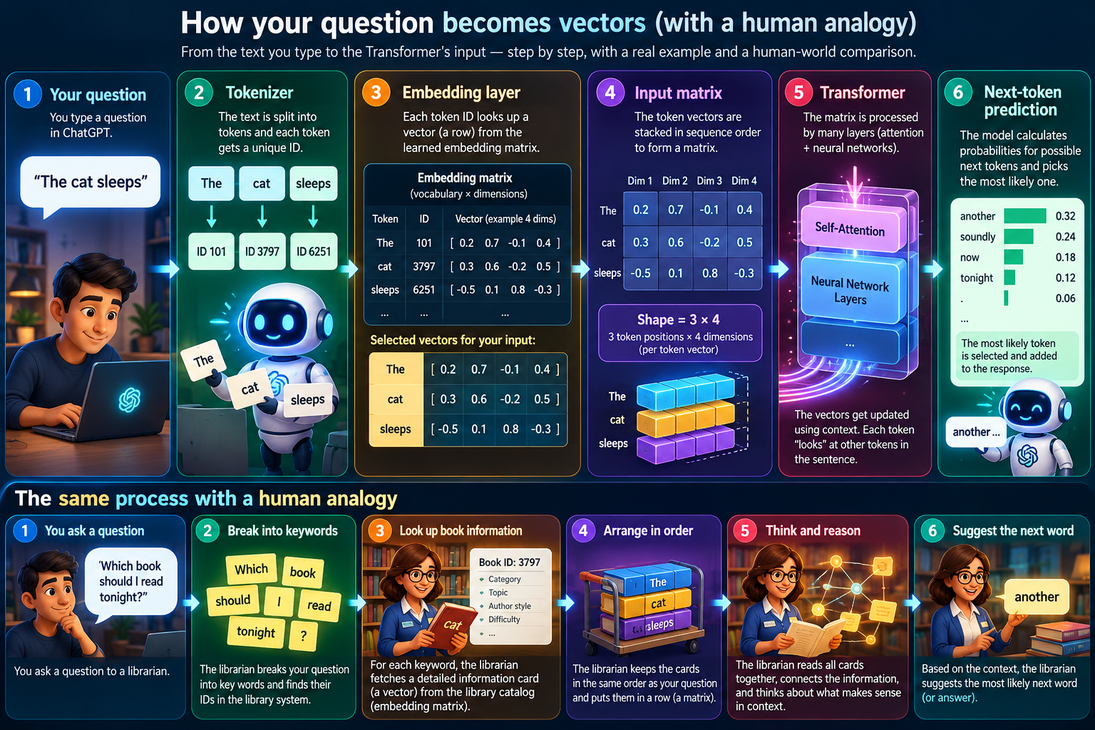
Every modern language model — BERT, GPT-4, LLaMA, T5 — shares one non-negotiable requirement before a single weight update can happen: text must be converted into numbers. Neural networks are mathematical machines. Every operation inside them — matrix multiplications, dot products, softmax activations, gradient descent — is defined only over real numbers. They have no concept of the string "cat", the word "democracy", or the sentence "the sky is blue".
This page answers the most fundamental question in NLP: why does text become numbers, and how does that conversion happen at each level — from character, to token, to integer ID, to a dense floating-point vector?
Human view
Words carry meaning through shared cultural context, syntax, metaphor, and pragmatics. A human reading "bank" uses surrounding words to resolve ambiguity in milliseconds.
Model view
A model receives a sequence of integer token IDs, maps each to a row in a learned embedding matrix, and performs matrix operations on the resulting sequence of floating-point vectors.
- Token ID — an integer index (e.g.
4127) that acts as an address in the vocabulary. It says which token this is, not what it means. - Embedding vector — a dense list of floating-point numbers (e.g.
[0.12, -0.41, 0.77, …]) that encodes learned semantic and syntactic properties. This is where meaning lives.
WhyFour reasons numbers are necessary
The requirement for numeric representation is not a limitation to work around — it is the foundation on which every learning algorithm is built. Here are the four pillars:
- Compute (matrix operations): Attention mechanisms, feed-forward layers, and embeddings all require matrix multiplication. You cannot multiply strings. A Transformer's self-attention is fundamentally $\text{softmax}\!\left(\frac{QK^\top}{\sqrt{d_k}}\right)V$ — every symbol here is a real-valued matrix.
- Learn (gradient descent): Training adjusts parameters by computing the gradient of a loss function with respect to those parameters. Gradients require derivatives, and derivatives require continuous numeric values. Discrete symbols like words have no natural gradient.
- Compare (dot products and distances): The model must assess how similar or related two pieces of text are. That comparison is geometric — cosine similarity, Euclidean distance — and geometry requires coordinates, not strings.
- Generalise (dense representations): Sparse representations (one word = one dimension) generalise poorly. Dense vectors allow the model to place similar concepts near each other in a continuous space, sharing learned properties across related tokens.
4127 does not mean "cat is more cat-like than token 4126". Meaning is encoded only in the embedding vector that the ID selects.
IntuitionThe airport record analogy
Imagine a global airport database. Every airport in the world has a 3-letter IATA code: JFK, LHR, NRT. Those codes are compact identifiers — analogous to token IDs. They tell the system which airport to look up, but the code itself says nothing about the airport's location, runway count, altitude, or passenger volume.
Behind each code is a full record: latitude, longitude, number of terminals, elevation, regional hub status, connection density, average delay. That rich record is the embedding vector. The code is an index; the record is the learned description.
Airport analogy:

  "cat"  →  token ID 4127  →  embedding [ 0.12, -0.41,  0.77,  0.23, -0.18, … ] (768 dims in BERT)
  "dog"  →  token ID 5863  →  embedding [ 0.09, -0.38,  0.81,  0.21, -0.15, … ]
  "car"  →  token ID 2912  →  embedding [-0.44,  0.22, -0.31, -0.52,  0.63, … ]

  cat and dog vectors are close  →  model learned they share properties (animals, domestic, etc.)
  car vector is far from both    →  model learned it belongs to a different region of meaning
This two-level design is deliberate. Token IDs are integers because integer indexing into an array is computationally free. The meaning-carrying work is entirely delegated to the embedding matrix, which is trained to place semantically similar tokens near each other in the vector space.
TheoryFour levels of text representation
Moving from raw text to model-ready input involves four distinct levels of abstraction, each solving a different problem:
| Level | What it is | Example for "cat" | Size | Expresses meaning? |
|---|---|---|---|---|
| Token | A unit of text — word, subword, or character, depending on the tokenizer | "cat" |
Variable-length string | Human-readable, but not numeric |
| Token ID | An integer index into the vocabulary table; uniquely identifies the token | 4127 |
1 integer per token | No — it is an address, not a score |
| One-hot vector | A binary vector of length V (vocab size) with a single 1 at position token_id | [0,0,…,1,…,0] at index 4127 |
V integers (e.g. 50,000) | No — no similarity between tokens |
| Dense embedding | A learned real-valued vector; the embedding matrix row selected by token_id | [0.12,-0.41,0.77,…] |
d floats (e.g. 768) | Yes — geometry encodes similarity |
In practice, modern neural networks skip the explicit one-hot step and directly implement the one-hot → dense multiplication as an embedding lookup (selecting a matrix row), which is computationally equivalent but far more efficient for large vocabularies.
How It WorksThe embedding lookup pipeline
Here is the concrete pipeline for turning a sentence into model-ready vectors:
"the cat sat" → ["the", "cat", "sat"]. The tokenizer splits text into units the vocabulary knows about.
[101, 4127, 2938]. This is a simple dictionary lookup.
4127 selects row 4127 of E, yielding a vector $\mathbf{x}_{4127} \in \mathbb{R}^d$.
[seq_len, d] — three 768-dimensional vectors for our three-token sentence. This is the input to the first Transformer layer.
The embedding matrix $E$ starts with random values and is updated during training via backpropagation. By the end of training, its rows encode the full semantic and syntactic knowledge the model has extracted from the training corpus. The matrix is essentially the model's entire vocabulary of learned concepts, stored as geometry in a $d$-dimensional space.
MathematicsFormalising the token → vector map
Let's be precise about the mathematics. The embedding layer defines a function:
$$E : \{0, 1, \ldots, V-1\} \rightarrow \mathbb{R}^d$$
where $V$ is the vocabulary size and $d$ is the embedding dimension. Concretely, $E$ is implemented as a matrix $\mathbf{E} \in \mathbb{R}^{V \times d}$, and the embedding of token $t_i$ is the $t_i$-th row:
$$\mathbf{x}_i = \mathbf{E}[t_i] \in \mathbb{R}^d$$
The key transition this formalises is discrete → continuous: token IDs are elements of a finite discrete set $\{0, \ldots, V-1\}$; embedding vectors are points in the continuous space $\mathbb{R}^d$. This is what makes gradient descent possible — you can take derivatives with respect to the entries of $\mathbf{E}$.
Worked ExampleTiny 5-token vocabulary, all levels shown
Use this small example to see all four representation levels side by side. Vocabulary of 5 tokens: the, cat, sat, dog, ran.
What can you observe from this toy table?
- ID 1 vs ID 3: The integers 1 and 3 say nothing about their relationship. But the dense vectors for
catanddogare very similar — their first dimension is high and positive for both, and their third dimension is negative for both. The model has learned they share properties. - sat vs ran: Both have high values in dimension 2 and 3. They are both verb-like. Their IDs (2 and 4) are completely uninformative about this.
- the: Very small values across all dimensions — as a function word, it has weak standalone semantics and sits near the origin in this toy space.
- One-hot is flat: Every token is equidistant from every other token in one-hot space. The cosine similarity between any two distinct one-hot vectors is exactly 0. Dense vectors break this symmetry by placing related tokens closer together.
VisualizeThe full pipeline as a flow diagram
The diagram below shows the complete transformation from raw text to the dense vectors that enter the first layer of a Transformer. Each arrow represents one stage of processing:
The critical bridge is the embedding matrix lookup (third arrow). Before that step, we are in the discrete world of integers. After that step, we are in the continuous world of real-valued vectors where all of the model's learned geometry lives.
The positional embedding added in the final step encodes where in the sequence each token appears — without it, the model would treat "cat sat" and "sat cat" identically.
CodeText-to-vector lookup in plain Python
This implementation shows every stage of the pipeline using only built-in Python — no NumPy, no PyTorch, no ML library. The goal is to make the mechanics transparent.
"""
Text-to-vector pipeline in plain Python.
Shows each stage: token → ID → (one-hot) → dense vector.
Does NOT learn or update the embedding table — that happens during training.
"""

# ── Vocabulary (token → integer ID) ─────────────────────────────────────────
vocab = {
    "the": 0,
    "cat": 1,
    "sat": 2,
    "dog": 3,
    "ran": 4,
}

# ── Toy embedding table (pre-trained / random initialisation) ────────────────
# Shape: [vocab_size, embedding_dim] = [5, 3]
# In real models this is learned from data. Here we use hand-crafted values
# that illustrate semantic clustering.
embedding_table = [
    [ 0.03, -0.02,  0.01],   # ID 0  → "the"   (function word, near origin)
    [ 0.85,  0.62, -0.44],   # ID 1  → "cat"   (animal, domestic)
    [-0.12,  0.78,  0.91],   # ID 2  → "sat"   (verb, stationary)
    [ 0.82,  0.59, -0.41],   # ID 3  → "dog"   (animal, domestic — close to cat)
    [-0.09,  0.77,  0.88],   # ID 4  → "ran"   (verb, motion — close to sat)
]

def text_to_ids(text: str) -> list[int]:
    """Step 1 & 2: tokenize (split on whitespace) and map to token IDs."""
    tokens = text.lower().split()
    ids = []
    for token in tokens:
        if token not in vocab:
            raise ValueError(f"Token '{token}' not in vocabulary")
        ids.append(vocab[token])
    return ids

def ids_to_vectors(ids: list[int]) -> list[list[float]]:
    """Step 3: embedding lookup — select the row for each ID."""
    # Equivalent to: one_hot @ embedding_table  (but O(n) not O(n*V))
    return [embedding_table[i] for i in ids]

# ── Pipeline ─────────────────────────────────────────────────────────────────
text = "the cat sat"

token_ids = text_to_ids(text)
print("Token IDs:", token_ids)           # [0, 1, 2]

vectors = ids_to_vectors(token_ids)
for tok, tid, vec in zip(text.split(), token_ids, vectors):
    print(f"  '{tok}' (ID {tid}) → {vec}")

# Output:
#   'the' (ID 0) → [0.03, -0.02, 0.01]
#   'cat' (ID 1) → [0.85, 0.62, -0.44]
#   'sat' (ID 2) → [-0.12, 0.78, 0.91]

# ── What this code does NOT do ───────────────────────────────────────────────
# 1. Learn vectors from data (no backprop, no gradient updates)
# 2. Handle subword tokenization (BPE / WordPiece / SentencePiece)
# 3. Add positional embeddings
# 4. Handle OOV tokens gracefully (would need [UNK] fallback)
# 5. Run in a neural network context (PyTorch: nn.Embedding does all of this)
What this covers
The complete token → ID → vector pipeline. Each stage is explicit so the mechanics are visible. The embedding lookup is a simple array index — fast and differentiable.
In PyTorch
nn.Embedding(vocab_size, d) wraps this exact lookup. During training, the embedding table rows are updated by gradient descent. At inference, it's a read-only lookup.
embedding_table[i] — array indexing. All the intelligence is in the values of that table, learned over millions of training steps.Hands-onInteractive pipeline explorer
Type a word from the toy vocabulary (the, cat, sat, dog, ran) and see the token ID and embedding vector at each stage.
CompareToken ID vs One-hot vs Dense embedding
Each representation solves a different problem. Understanding when to use which is essential for debugging and designing NLP systems.
| Property | Token ID | One-hot vector | Dense embedding |
|---|---|---|---|
| Type | Single integer | Binary vector of length V | Real-valued vector of length d |
| Size | 1 number (e.g. 4127) | V numbers (e.g. 50,000) | d numbers (e.g. 768) |
| Expresses similarity? | No — ID ordering is arbitrary | No — all pairs are equidistant | Yes — nearby vectors = similar meaning |
| Main role | Efficient index / lookup key | Conceptual bridge (rarely used explicitly) | Semantic representation for neural computation |
| Learned? | No — fixed by vocabulary construction | No — deterministic from ID | Yes — updated by gradient descent during training |
| Can be fed directly to a neural net? | Only as an index (not as a feature) | Technically yes, but impractically large | Yes — this is the standard input format |
ApplyWhere this bridge shows up in production
The text-to-vector conversion is not just an entry-point detail — it shapes how every downstream NLP system is designed and debugged.
Large Language Models
Every GPT-4, LLaMA, or Claude call starts here. Token IDs from the tokenizer index into a learned embedding matrix. The sequence of resulting vectors is what the Transformer stack actually processes. The "intelligence" emerges from learned geometry, not from the integer IDs.
Semantic search
Systems like Google's search or enterprise RAG pipelines encode queries and documents into dense vectors (using sentence-level or passage-level embeddings built on top of token embeddings). Retrieval is a nearest-neighbour search in vector space — impossible without the numeric representation.
Retrieval-Augmented Generation (RAG)
RAG systems store document chunks as dense vectors in a vector database (Pinecone, Weaviate, pgvector). At query time, the query is embedded into the same space, and the closest document vectors are retrieved. The shared embedding space makes comparison possible.
Text classifiers
A sentiment classifier, spam detector, or intent recogniser takes the embedding of the [CLS] token (or a pooled sentence embedding) and feeds it to a linear classification head. The vector is the only numeric representation of meaning available to that head.
LimitationsWhat numbers cannot capture
Converting text to vectors is powerful, but several important properties of language are either lost or distorted in this process:
- Numbers ≠ understanding: A vector that places
"cat"near"dog"does not mean the model "understands" what cats are. It means those tokens appeared in similar linguistic contexts during training. Correlation in context, not semantic comprehension. - Token ID is not a semantic score: Nothing about the integer 4127 says anything about the meaning of "cat". Models that inadvertently treat token IDs as meaningful numbers will learn incorrect relationships. This is a real bug in naive implementations.
- One-hot vectors encode no relationships: Before training, every token is equidistant from every other. The model must learn all semantic structure from scratch. Pre-trained embeddings (word2vec, GloVe, or embeddings from large LMs) warm-start this learning.
- Embeddings inherit training biases: If the training corpus contains societal biases, those biases are encoded into the geometric structure of the embedding space. The embedding of
"nurse"may be closer to"woman"than"doctor"in a biased corpus. - Similar vectors are evidence, not proof: High cosine similarity between two token vectors suggests they appear in similar contexts. It does not guarantee they are synonyms or that they are interchangeable in all contexts.
Feynman ChallengeCan you explain it simply?
Imagine explaining this to a smart friend who has never studied ML. Use the "puzzle-piece bridge" metaphor:
- Think of a word as a puzzle piece that needs to cross a bridge before it can enter a neural network.
- On the near side of the bridge: the word is a string of characters — the human side.
- The bridge has two lanes: first the word is stamped with a number (its token ID) — an efficient address. Then that address is used to retrieve a rich description (the embedding vector) from a learned table.
- On the far side: the model receives a list of coordinate points in a high-dimensional space — the machine side. All computation from this point forward is pure geometry and algebra.
- The learned table (embedding matrix) is the bridge's intelligence — it was trained to place words with similar meanings at similar coordinates.
Common misconceptions to tackle:
- "Token IDs encode meaning" — No. IDs are just row indices into the embedding table. The number 4127 has no semantic content. Only the vector at that row does.
- "One-hot vectors encode relationships" — No. Every token is equally distant from every other in one-hot space. The cosine similarity of any two distinct one-hot vectors is exactly 0.
- "I can use token IDs directly as model input features" — No (almost never). Feeding IDs directly to a linear layer treats them as numeric measurements, introducing false ordinal relationships. Always use the embedding lookup.
- "The vector IS the word" — Not quite. The vector is a learned approximation of the word's distributional properties in the training corpus. It captures what contexts the word appeared in, not what the word "is".
BuildCapstone mini-projects
🔨 Mini-Projects — cement every level of the pipeline
1 · Text-to-vector inspector CLI
Write a command-line script that takes a sentence as input and prints each token with its ID, its one-hot representation (abbreviated), and its embedding vector. Use a small hand-crafted vocabulary of 10–20 tokens. Make the output readable.
2 · Embedding table browser
Build a small HTML page or notebook that displays your toy embedding table with all four levels (token text, ID, one-hot, dense vector) side-by-side. Add a column showing the L2 norm of each vector and sort tokens by norm.
3 · Cosine similarity explorer
Write a function that takes two token names, looks up their embedding vectors, and computes cosine similarity. Test it on (cat, dog), (cat, ran), (sat, ran), (the, cat). Print a short explanation of why similar-meaning tokens have higher similarity.
SummaryThe complete picture
Here is everything this page covered, condensed to the essential points:
- Text → numbers is mandatory: Neural networks only operate on real-valued matrices. Strings, words, and tokens must be converted before any computation can happen.
- Four reasons: Compute (matrix ops), learn (gradient descent), compare (geometry), generalise (dense representation).
- Four levels: Token (text) → Token ID (integer) → One-hot (sparse binary) → Dense embedding (learned real-valued vector).
- Token ID is an address, not a score: It tells the model which row of the embedding matrix to retrieve. Adjacent IDs do not imply semantic similarity.
- Dense vectors are where meaning lives: The embedding matrix $\mathbf{E} \in \mathbb{R}^{V \times d}$ is learned from data. Its rows encode the geometric structure of language as distilled from the training corpus.
- The conversion is a bridge: Discrete → continuous. Before the bridge: combinatorial symbol space. After the bridge: differentiable geometric space.
| Representation | Type | Size | Semantic? | Role |
|---|---|---|---|---|
| Token | String | Variable chars | Human-readable | Human interface |
| Token ID | Integer | 1 number | No | Lookup index |
| One-hot | Binary vector | V numbers | No | Conceptual bridge |
| Dense embedding | Float vector | d numbers | Yes (learned) | Neural input |